Author: B J Wernick PrEng BScEng
Company: TechniSolve Software
Date: 17 February 2005
[Back]
This paper investigates the various methods that can be used to simulate the performance of the vapor compression refrigeration cycle.
The basis of the selected method is an object oriented model where each component in the system is developed and tested individually. As an example, I show the operation of the fin and tube model and develop some interesting solutions.
By making use of the polymorphic inheritance of the object model, the heat exchangers are interchangeable. For example, a DX coil would inherit properties from a fin and tube heat exchanger which in turn inherits its properties from a heat exchanger. The cycle is structured in such a way as to accept any type of heat exchanger. Therefore with no change to the solution module it is possible to change the cooling coil to a shell and tube, thereby making an air cooled chiller.
Finally, I present a case study of a reverse cycle heat pump. In air-conditioning systems, these are beneficial since waste can be used to produce useful heating. The problem is that there are conflicting criteria in the choice of the heat exchanger parameters. In this paper, I show how the design can be optimized and also indicate some of the consequences of poor heat exchanger selection.
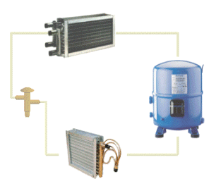
The vapor compression refrigeration cycle needs very little introduction. There are many installations around the world from small domestic heat pumps to giant multi-stage chillers generating chilled water for mine cooling. The principles of the cycle are identical. A refrigerant gas is compressed to a pressure where it is capable of releasing heat to a suitable sink. On expansion to a lower pressure, the cooled gas now has the ability to absorb heat from the source. In an air cooled air conditioner, this would mean cooling a room and rejecting the heat to ambient air. Figure 1 shows a typical air cooled air conditioner.

Figure 1. Air cooled air conditioner
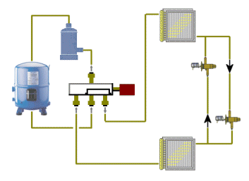
In a reverse cycle heat pump, the situation is the same. By using a change-over valve as shown in Figure 2, the roles of the evaporator and condenser can be swapped. The reverse cycle therefore refers to the changing role of the two heat exchangers. To avoid confusion, we now refer to the two parts as the indoor unit and the outdoor unit.

Figure 2. Reverse cycle heat pump
In light of the difficulty of finding a theoretical solution to the vapor compression cycle, it is a wonder that there are so many successful systems in the field. We will start here by describing a manual method that could be used to find a solution.
There are three primary components, the compressor, the evaporator and the condenser. A balance point is found when there is an energy balance between these three components. From the 1st law of thermodynamics, this is simply
| Qc = Qe + W | (1) |
|
where Qc = Condenser hear rejection, kW Qe = Cooling duty, kW W = Compressor power, kW |
The compressor performance relates to the mass flow of refrigerant gas. This is clearly a function of the compressor dimensions, running speed, suction specific volume and pressure ratio. For a reciprocating compressor, a simple model could be developed as follows.
| mr = ρs (V) ηvc | (2) |
|
where mr = Refrigerant mass flow, kg/s ρs = Density at inlet, kg/m3 V = Displacement rate, m3/s ηvc = Volumetric efficiency |
| W = mr dhi / ηi | (3) |
|
where W = Compressor power, kW mr = Refrigerant mass flow, kg/s dhi = Enthalpy change from Pe to Pc at constant entropy, kJ/kg ηi = Isentropic efficiency |
The problem with the above model is that compressor manufacturers do not publish efficiencies. What they do publish are tables of cooling duty and power consumption versus evaporating and condensing temperatures. For practical reasons, we therefore need to use these published performance figures as shown in figure 3.
| Models | Te |
+15°C | +10°C | +5°C | 0°C | -5°C | -10°C | -15°C | |||||||
| Tc | PF | PA | PF | PA | PF | PA | PF | PA | PF | PA | PF | PA | PF | PA | |
| MTZ 64 | 40°C | 25,992 | 4.90 | 21,218 | 4.68 | 17,064 | 4.39 | 13,480 | 4.05 | 10,418 | 3.68 | 7,830 | 3.27 | 5,666 | 2.85 |
| 50°C | 22,230 | 5.61 | 18,016 | 5.25 | 14,366 | 4.84 | 11,230 | 4.39 | 8,561 | 3.92 | 6,310 | 3.43 | - | - | |
| MTZ 72 | 40°C | 28,721 | 5.58 | 23,570 | 5.32 | 19,069 | 4.99 | 15,169 | 4.60 | 11,820 | 4.17 | 8,972 | 3.71 | 6,575 | 3.23 |
| 50°C | 24,668 | 6.39 | 20,107 | 5.97 | 16,137 | 5.50 | 12,709 | 4.99 | 9,773 | 4.45 | 7,279 | 3.89 | - | - | |
| MTZ 80 | 40°C | 31,994 | 6.39 | 26,391 | 6.09 | 21,475 | 5.70 | 17,196 | 5.26 | 13,503 | 4.76 | 10,343 | 4.23 | 7,667 | 3.69 |
| 50°C | 27,590 | 7.32 | 22,612 | 6.83 | 18,259 | 6.29 | 14,480 | 5.70 | 11,225 | 5.08 | 8,441 | 4.45 | - | - | |
| MTZ 100 | 40°C | 39,809 | 6.67 | 32,462 | 6.59 | 26,112 | 6.38 | 20,677 | 6.07 | 16,075 | 5.68 | 12,225 | 5.22 | 9,045 | 4.71 |
| 50°C | 33,872 | 7.97 | 27,417 | 7.66 | 21,867 | 7.24 | 17,144 | 6.75 | 13,165 | 6.19 | 9,850 | 5.59 | - | - | |
Figure 3. Extract from Maneurop Compressor Catalog showing MTZ Range based on R407C
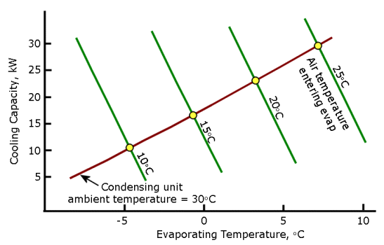
By combining the compressor performance with the condenser and evaporator performance curves, it is possible to plot a system balance chart as shown in figure 4.

Figure 4. Example of a system performance chart
This is a time consuming process, especially if you plan to change design parameters and probably explains why it is so seldom done. You must realize that you need the performance curves of the heat exchangers as well.
A better alternative would be to develop a simulation model. This will allow you to:
We showed earlier that the compressor performance could be developed to give the refrigerant mass flow for a given efficiency. In theory, this seems to be the correct approach but consider the source of the data. The efficiency would have to comply with the published performance data. If not, the model would be useless. So, why go to all the effort of building a theoretical model that would eventually be reduced to a curve fit?
The traditional way of dealing with this is to use a curve fit directly with the published figures. Clearly, some form of relationship is needed.
|
Qe = f (te, tc) Qc = f (te, tc) |
(4) |
|
where Qe = Cooling duty, kW Qc = Heat rejection, kW te = evaporating temperature, °C tc = condensing temperature, °C |
An inspection of a few compressor curves shows that a 2nd degree polynomial in both variables is a reasonable choice. This would take the form shown in equation (5).
| Z = a0 + a1X + a2X2 + a3Y + a4Y2 + a5XY + a6X2Y + a7XY2 + a8X2Y2 | (5) |
|
where ai are the coefficients calculated from a curve fit X and Y are the evaporating and condensing temperatures Z is the power, cooling duty or heat rejection, kW |
Clearly, not all of the terms of this polynomial would be significant but it makes no sense to simplify the equation since the appropriate equation would then be different for different compressors. Recently, a compressor selection computer program supplied by Maneurop, France included coefficients for this same polynomial.
The heat exchangers are another matter. There is no standard heat exchanger model. Increase the diameter of a shell and tube by 1 mm and you would have to cater for a different model! We therefore need to consider a suitable theoretical model.
For the mean time, we will ignore the problems with two-phase heat transfer on the outside of a cooling coil. The driving force for heat transfer is the temperature difference and the duty can be expressed as a fraction of the maximum possible duty.
| Q = ε Qmax | (6) |
|
where ε is the effectiveness Qmax = Cmin ITD Cmin = Minimum capacity rate, kW/K ITD = Inlet temperature difference, °C |
The advantage of this approach is that the effectiveness can be calculated from the basic dimensions and the flow configuration. The effectiveness of a counter-flow heat exchanger can be shown to obey the following relationship.
| ε = (1 - e(Cr (1-Ntu))) / (1 - Cr e(Cr (1-Ntu))) | (7) |
|
where Ntu = umber of transfer units = Uo Ao / Cmin Cr = Capacity ratio = Cmin / Cmax Uo = Overall heat transfer coefficient, W/m2°C Ao = Outside surface area, m2 Cmin = Minimum capacity rate, kW/K Cmax = Maximum capacity rate, kW/K |
The ITD is the temperature difference between the fluid inlet conditions. For example, in a shell and tube condenser, the ITD is the temperature difference between the condensing temperature and the water inlet temperature.
The above component models can now be combined and solved numerically.
The comprehensive approach would be to list all the variables and develop the same number of independent equations. This method would be applied with the detailed theoretical compressor model and would give the most freedom in solution. For example, you would be able to determine the size of the compressor cylinder in order to achieve a certain capacity. This would be of value to the compressor manufacturer but of limited use to the system designer. After all, the system designer would not normally be able to control the dimensions of the compressor in question.
There are a number of methods available to solve these systems but most are derived from the Newton-Raphson technique. Something worth mentioning here is that large non-linear systems are inherently unstable and often end up diverging.
Before diving in and solving a n-dimensional non-linear system, it is worth taking a look at the compressor polynomials. The coefficients are pre-calculated and therefore do not form part of the solution. This means that there are only two variables in the whole system. Given a value of te and tc, all other values are known. This includes the heat exchangers.
In this paper, we have adopted the curve-fit compressor model based on manufacturers performance data. The advantage is that the published figures incorporate efficiency, piston clearance, oil effects and heat losses from the casing.
By expressing the equations in terms of errors, it is now possible to find te and tc such that there is zero error.
| ee = Compressor Qe (te, tc)
- Evaporator Qe (te) ec = Compressor Qc (te, tc) - Condenser Qc (tc) |
(8) |
|
where ee is the cooling duty error ec is the heat rejection error |
In a real system, you would easily be able to make a good starting guess at te and tc. Using the previously selected temperatures, calculate the errors. The largest of these errors can now be minimized by adjusting te or tc.
Programming languages have taken a big step forward in 1985 when the object oriented paradigm started to become commercially available. Companies like Borland introduced hybrid versions of objects and functional language features in Pascal and C. In essence these two are similar, the only real difference being in the reserved words. Visual Basic to a lesser extent seems to have followed the trend. We see in the so called 3rd generation macro languages in excel and others similar structural features. Apart from dealing with the complexities of the multi-user operating system environments, there has not been much more development in language structure since the early introduction of objects. In this paper, we have used Delphi which is the Borland Pascal implementation.
The object oriented paradigm has made a huge impact in the writing of technical programs. The reason is that a numerical model can be developed to approximate the actual physical object. But it has further implications that are worth mentioning here. A feature called polymorphic inheritance allows you to create a hierarchy without having to write the code for each individual model.
Consider a practical example. A direct expansion cooling coil is a fin and tube heat exchanger. The appropriate hierarchy would then be as follows:
object HeatExchanger
Ao, Ai, HotFluid, ColdFluid...
object FinAndTube (HeatExchanger)
FinHeight, FinLength, FaceArea, AirFlow...
object DXCoil (FinAndTube)
Superheat, Solve...
object ACCoil (FinAndTube)
SubCooling, Solve...
object ShellAndTube(HeatExchanger)
D, L...
Since all heat exchangers have two fluids and a duty, these properties are placed at the heat exchanger level and are automatically inherited by the DX Coil. Not all heat exchangers have fins or airflow, so these properties belong in the FinAndTube object. Finally, you will see that the DXCoil and the ACCoil inherit from the FinAndTube and add the appropriate solution methods.
This technique models the real world so closely that it makes development and error detection easy, if that can be said about any programming.
The actual solution of the vapor compression cycle is now independent of the component type. In fact, the cycle component is not aware of the type of cycle it is solving.
object Cycle
Compressor, Evaporator, Condenser...
The Evaporator in the Cycle model is defined as a heat exchanger. This means that it could take on the characteristics of any type of heat exchanger at run time.
This means that an air-cooled chiller can be developed simply by changing the DX Coil to a Shell and Tube evaporator. This is the polymorphic part of the language. By sending the instruction Evaporator.Solve, the program automatically pulls in the correct solution method.
We will now define a typical air-cooled air-conditioner to deliver 20 kW of cooling.
| Ambient conditions | 30/20°C at 1700 m above sea level |
| Condensing temperature = 45°C | If we allow a 15°C temperature difference across the condenser. |
| The room set point | 23°C at 50% relative humidity |
| Airflow 1 m3/s with 12% fresh air | From a heat load calculation, you would know the air volume and the fresh air fraction |
| On-coil temperature is 23.8/16.3 C | Found by mixing the 12% ambient with the return air at room set point. |
| Evap coil: 533 mm high x 750 mm long |
Evaporator face velocity of 2.5 m/s From good design practice, we will choose a 4-row 12-fpi |
| Cond coil: 686 mm high x 1400 mm long | The condenser coil will be a 3-row 12-fpi and sized for 2.8 m/s face velocity. Airflow 2.69 m3/s |
| Design supply air temperature is 13°C | From the heat load calculations |
| Evaporating temperature of 6°C | Reasonable guess |
From the Maneurop catalog, we can now select a compressor that delivers 20 kW of cooling at 6/45°C.
In this case, a possible R22 compressor would be the Maneurop MT80. At 6/45°C, this compressor would give 20.7 kW
In practice, the balance point of the actual system will not be 6/45°C, it will depend on the simultaneous solution of each of the components at the on coil temperatures specified.
We have written a computer program that applies the practical method above, so now we can use this to find a solution.
The actual balance point of the MT80 compressor with the specified coils is 4.1/44.5°C. This would lead to a cooling duty of 19.4 kW and a heat rejection of 25.2 kW. This is easy to verify on the compressor catalog.
The next step is to check the duty of the heat exchangers.
| Condenser | Evaporator | |
| Heat transfer | ho = 0.065 Ui = 2.058 Ntu = 1.097 Qt = e x Qmax = 0.666 x 37.77 = 25.16 |
ho = 0.061 Ui = 3.531 Ntu = 0.919 Qt = e x Qmax = 0.601 x 32.30 = 19.42 |
| Air side | Qt = ma (hao - hai) = 2.530 (75.89 - 65.94) = 25.16 Qs = ma x Cpa (dbo - dbi) = 2.530 x 1.032 (39.6 - 30.0) = 25.16 |
Qt = ma (hao - hai) = 0.961 (32.27 - 52.47) = -19.42 Qs = ma x Cpa (dbo - dbi) = 0.961 x 1.027 (9.8 - 23.8) = -13.84 |
| Refrigerant side | Qt = mr x dh = 0.078 x 322 = 25.2 |
Qt = mr x dh = 0.118 x 164 = 19.4 |
Finding a balance point is tedious to do manually but checking the solution is easy. From the coil calculations, we see that in each case, the air side duty is equal to the refrigerant side duty and the heat transfer between refrigerant and air.
From the energy balance, the power is W = Qc - Qe = 25.2-19.4 = 5.8 kW.
In this example, we have assumed the coil sizes and did the calculations to find the actual balance point. The result shows a 4.1°C suction temperature that may be a bit low. Finding a new solution would entail a complete recalculation. To raise the suction temperature, you need to increase the size of the evaporator. At this point you can clearly see the benefit of having a software program to perform this task.
Recently, the reverse cycle heat pump is being offered more often than the "cooling only" option by suppliers. The advantage is that the cost of heating is about 25% of the electrical heating alternative.
We will now examine the effect of applying a reverse cycle to the above example. The roles of the evaporator and condenser change but we need to consider also the temperatures when heating is needed. The worst case could be at an ambient of 5°C and a room set point of 21°C. Keeping the same fresh air fraction, this would give an evaporator on-coil of 19.1/13.0°C.
The new balance point is now -2.6/44.9°C (SST/SDT) with a heat rejection of 19.8 kW.
If you have been involved in designing equipment of this type, you will recognize that the low suction temperature represents a problem since moisture in the outdoor air will freeze on the coil. A possible solution would be to sacrifice a bit of the heating and use some of the hot gas to raise the suction. In this case, it could work well since in South African conditions you normally only need about 1/3 of the cooling capacity for heating.
Another approach would be to increase the size of the outdoor coil. Since we now have an easy way to do these calculations, this would be easy to test. By changing the size of the outdoor coil to 686 mm high x 2000 mm wide 4-row 12-fpi, the heating mode suction raises to -0.6°C where you would probably get minimal icing on the coil. Under these conditions, the heating would be 21 kW. This revised outdoor coil design at cooling conditions would give a system cooling duty of 20.5 kW at 3.6/38.6°C (SST/SDT).
In order to find the balance point of a refrigeration system, you need to find a simultaneous solution between the compressor, the evaporator and the condenser. This can be done graphically by combining the components and plotting the system performance on a graph. The problem with this approach is that it does not cater for component design changes. Clearly, a computer model offers much advantage in the speed of solution but also in avoiding errors.
We have discussed a theoretical and a practical approach. Our preference was to adopt a pseudo-practical method where the heat exchangers are modeled in detail but the compressor is based on a curve fit of published data. The practical model is easy to apply numerically and can be extended to include all types of heat exchanger types.
In heat pump applications, it is essential that the balance point be determined under peak heating and cooling conditions. To find a suitable design, the designer would need to perform a number of system balances. The benefit of a numerical simulation to test these design changes is obvious. It is clear in the reverse cycle that the effect of local ambient conditions on the ideal design can not be ignored.
ASHRAE 2001 Fundamentals Handbook.
ASHRAE 2002 Refrigeration Handbook.
Maueurop Compressor Selection Program. Maneurop France.
Reay, D.A and Macmichael, D.B.A "Heat Pumps: Design and Applications", Pergamon Press, First Ed. 1979.
SAIRAC 2004 Technical Data Manual, Wernick B.J. Ed.
Stoecker, W.F. and Jones, J.W. "Refrigeration & Air Conditioning", 2nd Ed. McGraw Hill 1982.
Wernick, B.J. "Effectiveness method", RACA Journal, 2004.
Wernick, B.J. "RefSim Computer Program", Downloaded 2004 from www.coolit.co.za.
Copyright TechniSolve Software © 2004 All rights reserved